IMU and Wheel Odometry Dead Reckoning on SE(3)
Zhijian Qiao
This is an English translation of my Chinese article.
1. Introduction
IMU and wheel-odometry dead reckoning can be defined by its inputs and output:
- Input: IMU data (timestamps, acceleration, and angular velocity) and wheel-odometer data (timestamps and each wheel’s speed).
- Output: robot pose.
The technique is commonly used on wheeled robots to obtain a 2D pose. For robots operating outdoors, however, a 2D pose is often not enough. This post presents IMU and wheel-odometer dead reckoning on SE(3), using a smoother integration method to obtain a 3D pose.
2. Related work
- GR-Fusion: Multi-sensor Fusion SLAM for Ground Robots with High Robustness and Low Drift.
- Wheel-INS: A Wheel-Mounted MEMS IMU-Based Dead Reckoning System.
- A Micro Lie Theory for State Estimation in Robotics.
- State Estimation for Robotics, chapter 6.
3. Background
3.1 Time derivative of a rotation matrix
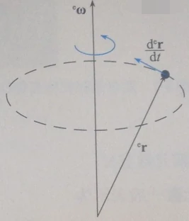
Figure from Inertial Navigation, as reproduced in the Chinese article.
As shown above, differentiating a 3D vector in global frame e gives:
\[\frac{\mathrm{d}^{\mathrm{e}} \mathbf{r}}{\mathrm{d} t}={ }^{\mathrm{e}} \boldsymbol{\omega} \times{ }^{\mathrm{e}} \mathbf{r}\]Write the cross product of two vectors as $\mathbf{a} \times \mathbf{b}=[\mathbf{a}]_{\times} \mathbf{b}$, where:
\[[\mathbf{a}]_{\times} \triangleq\left[\begin{array}{ccc} 0 & -a_{z} & a_{y} \\ a_{z} & 0 & -a_{x} \\ -a_{y} & a_{x} & 0 \end{array}\right]\]The 3D rotation matrix from body frame b to global frame e can be written:
\[\mathbf{R}_{\mathrm{b}}^{\mathrm{e}}=\left[\begin{array}{lll} { }^{\mathrm{e}} \mathbf{b}_{1} & { }^{\mathrm{e}} \mathbf{b}_{2} & { }^{\mathrm{e}} \mathbf{b}_{3} \end{array}\right]\]Here ${ }^{\mathrm{e}} \mathbf{b}_{1}$ represents body unit vector $\mathbf{b}_{1}$ in the global frame, so:
\[{ }^{\mathrm{e}} \mathbf{b}_{1}=\mathbf{R}_{\mathrm{b}}^{\mathrm{e}} \mathbf{b}_{1}\]Differentiating gives:
\[\frac{\mathrm{d} \mathbf{R}_{\mathrm{b}}^{\mathrm{e}}}{\mathrm{d} t}=\frac{d\left[\begin{array}{lll} { }^{e} \mathbf{b}_{1} & { }^{e} \mathbf{b}_{2} & { }^{e} \mathbf{b}_{3} \end{array}\right]}{d t}=\left[\begin{array}{lll} { }^{e} \boldsymbol{\omega} \times{ }^{e} \mathbf{b}_{1} & { }^{e} \boldsymbol{\omega} \times{ }^{e} \mathbf{b}_{2} & { }^{e} \boldsymbol{\omega} \times{ }^{e} \mathbf{b}_{3} \end{array}\right]\]Continuing the derivation:
\[\begin{array}{l} \frac{\mathrm{dR}_{\mathrm{b}}^{\mathrm{e}}}{\mathrm{dt}}=\left[\left(\mathrm{R}_{\mathrm{b}}^{\mathrm{e} \mathrm{b}} \omega\right) \times\left(\mathrm{R}_{\mathrm{b}}^{\mathrm{c}} \mathrm{b}_{1}\right) \quad\left(\mathrm{R}_{\mathrm{b}}^{\mathrm{e} \mathrm{b}} \omega\right) \times\left(\mathrm{R}_{\mathrm{b}}^{\mathrm{e}} \mathrm{b}_{2}\right) \quad\left(\mathrm{R}_{\mathrm{b}}^{\mathrm{e} \mathrm{b}} \omega\right) \times\left(\mathrm{R}_{\mathrm{b}}^{\mathrm{e}} \mathrm{b}_{3}\right)\right] \\ =\left[\mathrm{R}_{\mathrm{b}}^{\mathrm{e}}\left({ }^{\mathrm{b}} \omega \times \mathrm{b}_{1}\right) \quad \mathrm{R}_{\mathrm{b}}^{\mathrm{e}}\left({ }^{\mathrm{b}} \omega \times \mathrm{b}_{2}\right) \quad \mathrm{R}_{\mathrm{b}}^{\mathrm{e}}\left({ }^{\mathrm{b}} \omega \times \mathrm{b}_{3}\right)\right] \\ =\mathrm{R}_{\mathrm{b}}^{\mathrm{e}}\left[{ }^{\mathrm{b}} \omega \times \mathrm{b}_{1} \quad{ }^{\mathrm{b}} \omega \times \mathrm{b}_{2} \quad{ }^{\mathrm{b}} \omega \times \mathrm{b}_{3}\right] \\ =\mathrm{R}_{\mathrm{b}}^{\mathrm{e}}\left[{ }^{\mathrm{b}} \omega\right]_{\mathrm{x}} \end{array}\]Using $[\mathbf{Ra}]_{\times}=\mathbf{R}[\mathbf{a}]_{\times}\mathbf{R}^T$, we can also write this as:
\[\frac{\mathrm{dR}_{\mathrm{b}}^{\mathrm{e}}}{\mathrm{dt}}=\left[{ }^{\mathrm{e}} \boldsymbol{\omega}\right]_{\mathrm{x}}\mathrm{R}_{\mathrm{b}}^{\mathrm{e}}\]4. Method
4.1 Midpoint integration for dead reckoning
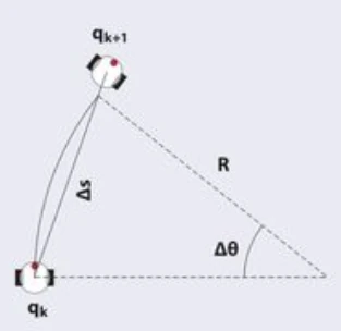
Figure from Camera–Odometry Calibration, as reproduced in the Chinese article.
Most of this section comes from Calibration Series II: Camera–Odometry Calibration in Practice.
The body motion equation using wheel encoders is:
\[\left[\begin{array}{c} \dot{\theta} \\ \dot{\mathbf{p}} \end{array}\right]=\left[\begin{array}{cc} 1 & \mathbf{0}_{1,2} \\ \mathbf{0}_{2,1} & \mathbf{R}(\theta)_{2,2} \end{array}\right]\left[\begin{array}{c} \omega \\ \mathbf{v}_{2,1} \end{array}\right]\]Here $\theta$ and $p$ are the body’s yaw and position in the 2D world frame; $R(\theta)$ is the 2D rotation; $v$ is body velocity, including forward and lateral components; and $\omega$ is angular velocity. Assuming no slip, the lateral velocity is zero, so:
\[\left[\begin{array}{c} \dot{\theta} \\ \dot{x} \\ \dot{y} \end{array}\right]=\left[\begin{array}{ccc} 1 & 0 & 0 \\ 0 & \cos (\theta) & -\sin (\theta) \\ 0 & \sin (\theta) & \cos (\theta) \end{array}\right]\left[\begin{array}{c} \omega \\ v_{x} \\ 0 \end{array}\right]=\left[\begin{array}{c} \omega \\ \cos (\theta) v_{x} \\ \sin (\theta) v_{x} \end{array}\right]\]Forward velocity $v_x$ and angular velocity $\omega$ can be expressed in terms of left and right wheel speeds $\omega_L$ and $\omega_R$, wheel radii $r_L$ and $r_R$, and wheel separation $b$. The latter three, $r_L$, $r_R$, and $b$, are the wheel-odometer intrinsic parameters:
\[\begin{aligned} v &=\left(\omega_{L} r_{L}+\omega_{R} r_{R}\right) / 2 \\ \omega &=\left(\omega_{R} r_{R}-\omega_{L} r_{L}\right) / b \end{aligned}\]Midpoint integration is a common way to integrate wheel odometry:
\[\left[\begin{array}{l} \theta_{t+1} \\ x_{t+1} \\ y_{t+1} \end{array}\right]=\left[\begin{array}{l} \theta_{t} \\ x_{t} \\ y_{t} \end{array}\right]+\left[\begin{array}{c} \omega \Delta t \\ \cos \left(\theta_{t}+\frac{\omega \Delta t}{2}\right) v_{x} \Delta t \\ \sin \left(\theta_{t}+\frac{\omega \Delta t}{2}\right) v_{x} \Delta t \end{array}\right]\]It uses the mean of the angles before and after motion when integrating translation.
4.2 Closed-form integration on SE(3)
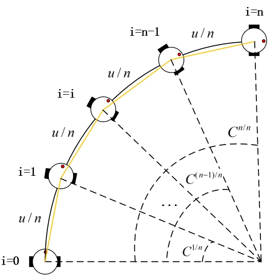
Figure from the Chinese article.
Let w be the world frame, p the previous frame, and c the current frame. We seek:
\[\mathrm{T}_{\mathrm{c}}^{\mathrm{w}}=\mathrm{T}_{\mathrm{p}}^{\mathrm{w}}*\mathrm{T}_{\mathrm{c}}^{\mathrm{p}}\]Here $\mathrm{T}_{\mathrm{c}}^{\mathrm{p}}$ is the quantity to solve for. In the figure, the robot travels at velocity v for a distance v·t = u. Integrating angular velocity gives the rotation matrix $\mathrm{C}_{\mathrm{c}}^{\mathrm{p}}$, abbreviated $\mathrm{C}$. Divide the motion into n parts and let n tend to infinity:
\[\mathrm{T}_{\mathrm{c}}^{\mathrm{p}}=\lim _{n \rightarrow \infty}\left(\prod_{i=0}^{i=n-1}\left[\begin{array}{cc} C^{\frac{1}{n}} & \frac{1}{n} u \\ 0 & 1 \end{array}\right]\right) \\ \begin{aligned} &=\lim _{n \rightarrow \infty}\left[\begin{array}{cc} C^{\frac{1}{n}}{ }^{* \mathrm{n}} & \sum_{\mathrm{i}=0}^{\mathrm{n-1}} \frac{1}{\mathrm{n}} C^{\frac{1}{\mathrm{n}} * \mathrm{i}}u \\ 0 & \mathrm{1} \end{array}\right] \\ &=\left[\begin{array}{cc} C & \int_{0}^{1} C^{\alpha} \mathrm{d} \alpha *\mathrm{u} \\ 0 & 1 \end{array}\right] \end{aligned}\]where:
\[\begin{aligned} \boldsymbol{J}= \int_{0}^{1} \boldsymbol{C}^{\alpha} \mathrm{d} \alpha &=\int_{0}^{1} \exp \left(\boldsymbol{\phi}^{\wedge}\right)^{\alpha} \mathrm{d} \alpha=\int_{0}^{1} \exp \left(\alpha \phi^{\wedge}\right) \mathrm{d} \alpha \\ &=\int_{0}^{1}\left(\sum_{n=0}^{\infty} \frac{1}{n !} \alpha^{n}\left(\phi^{\wedge}\right)^{n}\right) \mathrm{d} \alpha=\sum_{n=0}^{\infty} \frac{1}{n !}\left(\int_{0}^{1} \alpha^{n} \mathrm{~d} \alpha\right)\left(\phi^{\wedge}\right)^{n} \\ &=\sum_{n=0}^{\infty} \frac{1}{n !}\left(\left.\frac{1}{n+1} \alpha^{n+1}\right|_{\alpha=0} ^{\alpha=1}\right)\left(\phi^{\wedge}\right)^{n}=\sum_{n=0}^{\infty} \frac{1}{(n+1) !}\left(\phi^{\wedge}\right)^{n}\\ &=\frac{\sin \phi}{\phi} \mathbf{1}+\left(1-\frac{\sin \phi}{\phi}\right) \boldsymbol{a} \boldsymbol{a}^{\mathrm{T}}+\frac{1-\cos \phi}{\phi} \boldsymbol{a}^{\wedge} \end{aligned}\]It happens that $\boldsymbol{J}$ is the left Jacobian of rotation matrix $\mathrm{C}$. Here $\phi=|\phi|$ is the rotation angle and $a=\phi /| \phi|$ is the unit rotation axis. The final form of $\mathrm{T}_{\mathrm{c}}^{\mathrm{p}}$ is therefore:
\[\mathrm{T}_{\mathrm{c}}^{\mathrm{p}}=\left[\begin{array}{cc} C & \boldsymbol{J}\mathrm{u} \\ 0 & 1 \end{array}\right]\]A few practical points:
- An IMU generally provides acceleration as well as angular velocity. We can use IMU State Estimation: Quaternion Kinematics for ESKF to obtain a better rotation estimate.
- The wheel-odometer and IMU frames need not coincide, so transform wheel velocity into the IMU frame first.
- The wheel odometer and IMU generally sample at different rates; interpolate between measurements. Linear interpolation is usually sufficient.