PnP from Scratch: DLT, RANSAC, and Gauss–Newton
Zhijian Qiao
This is an English translation of my Chinese article.
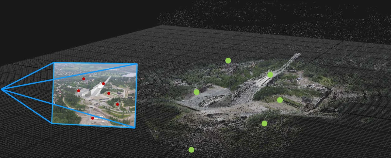
PnP illustration from slides by Trym Vegard Haavardsholm, as reproduced in the Chinese article.
Introduction
Normally, I would not need to implement PnP by hand, and I expect the same is true for you. But an ELEC5660 assignment prohibited OpenCV, and another student had raised the bar, so I sat down and wrote it properly. VNAV is another good course on the subject.
The figure shows the PnP problem: given points $(X,Y,Z,1)$ in space and their corresponding image pixels $(u,v,1)$, estimate the camera pose. In visual SLAM, for example, we can establish the world frame at the first frame and use stereo matching to obtain N 3D points $P_0$ and their pixels $p_0$. At frame K, we find pixels $p_0$ matched to $p_k$. These N 2D–3D correspondences let us estimate the camera pose at frame K in the world frame.
We can formulate the problem as:
\[\min _{\mathbf{R} \in \mathrm{SO}(3), \mathbf{t} \in \mathbb{R}^3} \sum_{i=1}^N \min \left(\left\|p_i-\pi\left(\mathbf{R} P_i^w+\mathbf{t}\right)\right\|^2, \bar{c}^2\right)\](1)
Here R and t are the rotation and translation to optimize. They transform a point from the world frame to the camera frame, so a more precise notation would be $(R_{cw},t_{cw})$. Each $(p_i,P_i^w)$ is a 2D–3D correspondence, and N is the number of correspondences. The camera projection function $\pi$ first divides the camera-frame point $P_i^c$ by $Z^c$ to obtain normalized coordinates, then multiplies by the intrinsic matrix K to obtain pixel coordinates. The threshold $\bar{c}$ distinguishes inliers from outliers. Its unit is pixels, as the quantity compared with it shows; one might choose five pixels depending on the application.
This is truncated least squares, a common way to account for outliers. It differs from ordinary least squares: an implicit indicator for whether a correspondence is an inlier is also being optimized. The problem therefore combines continuous and combinatorial optimization. I will not go deeply into optimal algorithms here; instead, I will use the classic and practical RANSAC framework. The code is at qiaozhijian/PnP-Solver.
DLT
DLT stands for direct linear transform. As its name suggests, we construct a linear equation and use it to solve PnP directly. For one 2D–3D correspondence:
\[p_i=\pi\left(\mathbf{R} P_i^w+\mathbf{t}\right)\]Denoting the point in normalized coordinates by $p^n_i$, we can write:
\[Z^{c} p_i^{n}=\mathbf{R} P_i^w+\mathbf{t}\](2)
This form is useful because an implementation will usually undistort pixels first:
cv::undistortPoints(pts_2, un_pts_2, K, D);
The output un_pts_2 is in normalized coordinates. Undistortion first uses the inverse of K to project pixels back to normalized coordinates, then removes distortion there using D. To return to pixels, we would project with K again. Here we can skip that step and replace the 2D pixel–3D correspondence with a normalized 2D–3D correspondence, as in equation (2).
DLT relaxes the original problem again. R belongs to SO(3), a non-convex set, making the optimization non-convex. DLT represents R as a 3×3 matrix and drops the SO(3) constraint. The space grows from three degrees of freedom to nine; the domain becomes convex, but more correspondences are needed to constrain the problem. Rewriting equation (2), we obtain:
\[Z^c\left(\begin{array}{l} x \\ y \\ 1 \end{array}\right)=\left(\begin{array}{llll} h_1 & h_2 & h_3 & h_4 \\ h_5 & h_6 & h_7 & h_8 \\ h_9 & h_{10} & h_{11} & h_{12} \end{array}\right)\left(\begin{array}{c} X \\ Y \\ Z \\ 1 \end{array}\right)\](3)
We have combined R and t into an augmented 3×4 matrix and now solve for 12 variables. The equation yields three equations, but one follows from the other two, so eliminate it to obtain:
\[\begin{aligned} &\boldsymbol{h}_1^T \boldsymbol{P}-\boldsymbol{h}_3^T \boldsymbol{P} x=0\\ &\boldsymbol{h}_2^T \boldsymbol{P}-\boldsymbol{h}_3^T \boldsymbol{P} y=0 \end{aligned}\]Bold $\boldsymbol{h}$ denotes a row of H. The unknowns are $\boldsymbol{h}_1,\boldsymbol{h}_2,\boldsymbol{h}_3$, twelve numbers in total. Each match supplies two constraints, so we need at least six nondegenerate matches. The Chinese article says that three coplanar points cause degeneracy; any three points are coplanar, so the relevant planar degeneracy is that the 3D points used by this DLT formulation all lie on a plane. In practice there are usually far more; as we will see, a solver requiring only three can be preferable in RANSAC. For N matches, we can construct an overdetermined system: it has more rows than columns, or more constraints than unknowns. A stable solution requires appropriate matrix rank:
\[\left(\begin{array}{ccc} \boldsymbol{P}_1^T & 0 & -x_1 \boldsymbol{P}_1^T \\ 0 & \boldsymbol{P}_1^T & -y_1 \boldsymbol{P}_1^T \\ \vdots & \vdots & \vdots \\ \boldsymbol{P}_N^T & 0 & -x_N \boldsymbol{P}_N^T \\ 0 & \boldsymbol{P}_N^T & -y_N \boldsymbol{P}_N^T \end{array}\right)\left(\begin{array}{c} \boldsymbol{h}_1 \\ \boldsymbol{h}_2 \\ \boldsymbol{h}_3 \end{array}\right)=0 \rightarrow Ax=0\]There are several ways to understand the classic $Ax=0$ problem. Here is one [2, 3]. The solution’s scale is arbitrary: multiplying by any λ leaves the equation unchanged. Multiplication by zero produces a degenerate answer, so impose $\|x\|_2=1$. We now have a quadratic optimization problem with an equality constraint:
\[\min \left(\|A x\|_2\right), \quad\|x\|_2=1\]Decompose A with SVD. By orthogonality:
\[\|A x\|=\left\|U D V^T x\right\|=\left\|D V^T x\right\|\]Let $y=V^T x$; the problem becomes $\min (\|D y\|),\|y\|=1$. If D is diagonal with singular values in descending order, the optimal solution is $y=[0,0, \cdots, 1]^T$. Since $y=V^T x$, the optimal x is the column of V, or right singular vector, corresponding to the smallest singular value.
We now have the optimal $(\boldsymbol{h}_1,\boldsymbol{h}_2,\boldsymbol{h}_3)$, but we are not done. It need not satisfy either the physical camera-projection constraint or the SO(3) constraint; recall that an arbitrary scale λ is possible.
First, substitute $(\boldsymbol{h}_1,\boldsymbol{h}_2,\boldsymbol{h}_3)$ back into equation (3) and check whether $Z^c$ is positive: a camera can see only points in front of it. Otherwise, multiply $(\boldsymbol{h}_1,\boldsymbol{h}_2,\boldsymbol{h}_3)$ by −1. Next, take the H matrix formed by $(\boldsymbol{h}_1,\boldsymbol{h}_2,\boldsymbol{h}_3)$ and project its first three columns $H_R$ onto SO(3), finding R that minimizes $\|R-H_R\|_F=\sqrt{\operatorname{tr}((R-H_R)^T(R-H_R))}$. The closing parenthesis in this Frobenius-norm expression has been corrected in translation. We can first solve the related orthogonal Procrustes problem for an orthogonal matrix, then obtain a rotation matrix. More specifically:
\[\begin{aligned} & \min \left\|R-U \Sigma V^T\right\|_F^2=\min \operatorname{tr}\left[\left(R-U \Sigma V^T\right)^T\left(R-U \Sigma V^T\right)\right] \\ & =\operatorname{tr}\left[R^T R+\left(U \Sigma V^T\right)^T U \Sigma V^T-2 R^T U \Sigma V^T\right] \end{aligned}\]Dropping terms independent of R gives:
\[\max \operatorname{tr}\left(R^T U \Sigma V^T\right)\]Using the cyclic trace identity $tr(ABC)=tr(CAB)$ and setting $Z=V^TR^TU$ gives:
\[\operatorname{tr}\left(R^T U \Sigma V^T\right)=\operatorname{tr}(Z\Sigma)=\sum_1^3{z_{ii}*\sigma_i}\leq\sum_1^3{\sigma_i}\]R, V, and U are orthogonal, giving the final inequality. The optimum is reached when Z is the identity, so:
\[R^T=V*U^T \rightarrow R=U*V^T\]There is one more detail. R is now orthogonal, but we need a right-handed rotation with determinant +1, not −1. If the determinant is negative, negate the last column of V and recompute R.
To find translation t, view the projection of H to (R, t) as multiplication by a scale λ. Estimate λ from the optimized R: its first column has unit norm, whereas the first column of the original H generally does not. The reciprocal of that original norm gives a rough estimate of λ. Multiply the translation by it to recover a scaled translation. See solvePnPbyDLT in the repository for this part.
A calibration board introduces a degenerate case: its 3D points all lie on one plane. Set z = 0, and the measurements no longer constrain H’s third column. Remove that column and derive the equations again. To recover R, its third column is still needed; one can obtain it from the cross product of the first two columns.
RANSAC
RANSAC is a familiar way to remove outliers. Once only inliers remain, equation (1) becomes ordinary least squares. RANSAC seeks maximum consensus: inliers agree with one another, while outliers generally do not. A consensus set contains mutually consistent elements. The approach succeeds when the true inlier set is the largest such set.
It is not quite correct to say that RANSAC cannot handle more than 50% outliers. Suppose just 1% of observations are inliers, with only three matching pairs, and the remaining 99% are mutually inconsistent outliers. The largest consensus set still has three elements; with enough iterations, RANSAC can find it. But if an outlier consensus set has more than three elements, RANSAC can fail. Repeated structures in real scenes can cause this. Such outliers are called adversarial; the usual assumption is that outliers are generic, random, and mutually inconsistent.
The steps are:
- Randomly select six points and use DLT to estimate the pose.
- Test the reprojection error of every correspondence against that pose. Set a threshold, such as five pixels; points below it are inliers, or members of the pose’s consensus set. Count them.
- Repeat steps 1–2. Always sample in step 1 from the full set, not the inliers found in step 2; sample with replacement across iterations.
- Stop when the inlier set is large enough, for example more than 50% of all observations, or when an iteration limit such as 1,000 is reached.
A key improvement is to reduce the minimum number of points needed by the model solver. If we can solve PnP using three points instead of six, RANSAC is more likely to find the right answer, or reaches a given success probability faster. See [4] for the derivation and solvePnPbyRANSAC for the code.
Gauss–Newton
Gauss–Newton is an optimization method in the gradient-descent family. Once we specify the residual and Jacobian, we can use its framework to solve the problem. The code defines the residual according to equation (2), as reprojection error on the normalized plane. The Jacobian can be derived similarly to section 7.7.3 of [1].
See solvePnPbyGaussianNewton for this part. Gradient-based methods depend on initialization, so we usually first obtain a rough solution using DLT and then refine it with Gauss–Newton.
Experiments
To compare the implementations, I ran an ablation with DLT, DLT + RANSAC, and DLT + RANSAC + Gauss–Newton. A virtual camera generated the data, and I added noise to the 2D pixels and 3D points. To test outlier robustness, I also added outliers with probability 0.2. I compared these three settings with OpenCV’s solvePnP and solvePnPRansac:
PnP Benchmark with 0 outlier ratio
Method: OPENCV, rotation error 0.303949 deg, translation error 0.131297
Method: OPENCV_RANSAC, rotation error 0.144112 deg, translation error 0.0910249
Method: DLT, rotation error 0.142964 deg, translation error 0.0931654
Method: DLT_RANSAC, rotation error 0.188459 deg, translation error 0.219939
Method: GAUSS_NEWTON, rotation error 0.194367 deg, translation error 0.157812

PnP Benchmark with 0.2 outlier ratio
Method: OPENCV, rotation error 119.313 deg, translation error 2.72919e+07
Method: OPENCV_RANSAC, rotation error 0.163613 deg, translation error 0.0977965
Method: DLT, rotation error 148.23 deg, translation error 105.087
Method: DLT_RANSAC, rotation error 0.271609 deg, translation error 0.252496
Method: GAUSS_NEWTON, rotation error 0.208845 deg, translation error 0.155049
Our DLT implementation works reasonably well without outliers. RANSAC helps reject them, and Gauss–Newton can further refine the result. In practice I recommend OpenCV’s implementation. I do not recommend using my code for a course assignment—trust me, the teaching assistants will find out. You can use it as a reference and acknowledge it in your report.
References
- Fourteen Lectures on Visual SLAM.
- Visual SLAM: PnP with DLT.
- Solving Overdetermined Equations with SVD.
- Konstantinos G. Derpanis, Overview of the RANSAC Algorithm.