Understanding and Implementing KLT Optical Flow
Zhijian Qiao
This is an English translation of my Chinese article on Zhihu.
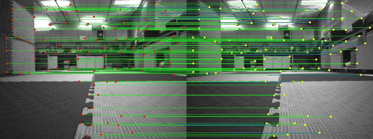
KLT optical flow. In the right image, yellow shows OpenCV’s tracks and blue shows my implementation. They overlap so closely that it is hard to tell them apart.
Introduction
I did not actually need to implement KLT optical flow from scratch, even though I was taking ELEC5660. I misread the assignment, just as I once misread a question on the college entrance exam and lost 20 points. Counting the effect on my state of mind, I think calling it 40 points is fair. Anyway, everything happens for the best. The assignment took a few extra days, but for a free and useless soul like me, that is no big deal.
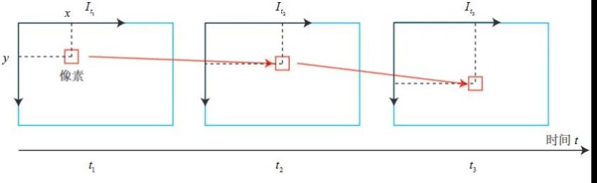
The LK optical-flow method. Lucas comes first in the paper’s author order. Figure from [1].
As shown above, optical flow, or sparse optical flow in this post, starts with feature points in image $I$, such as Tomasi corners. We find the pixel positions in image $J$ that correspond to the same 3D points. The process works entirely from image appearance, so it does not need the intrinsic matrix $K$ or the pose $R,t$. By analogy, the flow between two point clouds can be called scene flow.
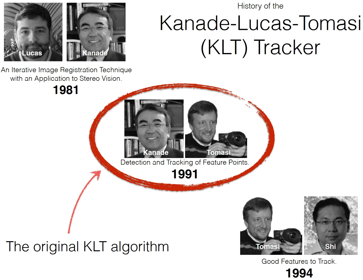
A history of the KLT name.
This post focuses on KLT optical flow. Kanade and Lucas proposed the optical-flow algorithm, and corners generally work well for tracking. Combining it with Tomasi corners gives us the KLT sparse optical-flow tracker. Code: KLT-Optical-Flow.
KLT Tracker
Brightness constancy is the basic assumption behind KLT: the pixel intensity of the same 3D point stays constant across images. For a pixel $p$ in image $I$, we want to find the corresponding pixel $p^\prime$ in image $J$. Under brightness constancy, we do not need to estimate the depth of $p$, recover the relative pose between the images, and project the 3D point to obtain $p^\prime$. We can instead search near $p$ in image $J$ for a pixel $p^\prime$ with similar intensity. Let
\[p^\prime=p+\Delta d.\]Our goal is to estimate $\Delta d$. The flow of a single pixel cannot be determined reliably. Even if it is very discriminative and the experimental conditions are ideal, noise can make it hard to distinguish from its neighbors. We therefore track using local information. This introduces the second assumption, surface markings: many surface markings exist in the real world, so all pixels in an image window follow the same transformation, such as the same $\Delta d$.
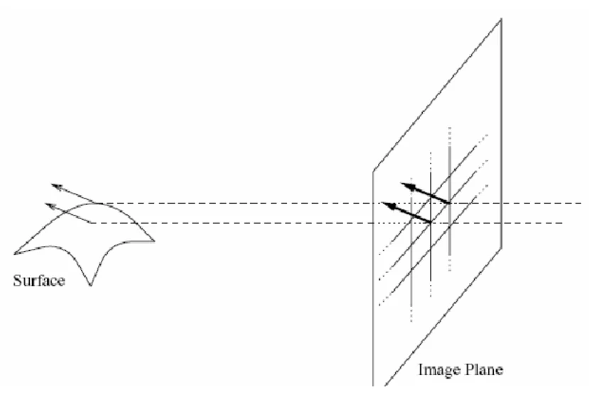
The surface markings assumption.
This assumption is strict. The part of the scene covered by a window may not be smooth, and its pixels may not even belong to the same object. We can add an affine transformation $A$:
\[p^\prime=p+Ap_w+\Delta d.\]Then pixels in the window have different optical flows, $Ap_w+\Delta d$, where $p_w$ is the position of $p$ within the window. The original author [3] also argues that, when the world is known to be rigid, the risks of over-parameterization can outweigh the benefits of a richer model; fewer parameters can be reliable for a small window. In this post we assume equal flow within a window, so $p^\prime=p+\Delta d$ for every pixel in it.
Let $I$ be the source image and $J$ the target image. A feature point in the source is $p=(u,v)$, its local window is $\mathcal{W}$, and the unknown is $\Delta d$. Under brightness constancy and the surface markings assumption, for any pixel $p_i$ in $\mathcal{W}$,
\[J(p_i+\Delta d)=I(p_i)+n(p_i). \tag{1}\]Here $n(p_i)$ is image noise with a zero-mean Gaussian distribution. We can therefore define the objective
\[\epsilon=\int_{\mathcal{W}}\left[J\left(p_i+\Delta d\right)-I\left(p_i\right)\right]^2 w_i\,dp_i. \tag{2}\]The weight $w_i$ for each pixel in the window can follow a Gaussian distribution. Alternatively, following [4], set
\[w_i=\frac{1}{\|J^{\prime}(p_i)-I^{\prime}(p_i)\|_2}. \tag{3}\]A pixel receives a larger weight if its gradients in the two images are similar.
To solve (2), the integral over $\mathcal{W}$ represents summation over the window. We can linearize $J(p_i+\Delta d)$ in this unconstrained quadratic optimization problem:
\[\epsilon=\int_{\mathcal{W}}\left[J\left(p_i\right)+g_i^T\Delta d-I\left(p_i\right)\right]^2 w_i\,dp_i. \tag{4}\]Here $g_i\in\mathbb{R}^{2\times1}$ is the gradient of image $J$ at $p_i$. At the optimum, the derivative of the objective with respect to $\Delta d$ is zero:
\[\begin{aligned} \int_{\mathcal{W}}[J(p_i)+g_i^T\Delta d-I(p_i)]g_iw_i\,dp_i &= 0, \\ \int_{\mathcal{W}}[w_ig_i^T\Delta d\,g_i]dp_i &= \int_{\mathcal{W}}w_i[I(p_i)-J(p_i)]g_i\,dp_i, \\ \left(\int_{\mathcal{W}}w_ig_ig_i^T\,dp_i\right)\Delta d &= \int_{\mathcal{W}}w_i[I(p_i)-J(p_i)]g_i\,dp_i. \end{aligned} \tag{5}\]Let
\[H=\int_{\mathcal{W}}w_ig_ig_i^T\,dp_i, \qquad b=\int_{\mathcal{W}}w_i[I(p_i)-J(p_i)]g_i\,dp_i.\]Solving the two-variable linear system $H\Delta d=b$ gives $\Delta d$.
Advanced KLT Tracker
Iterative refinement
We used a first-order Taylor expansion between (2) and (4). It is already an imperfect approximation for an ordinary nonlinear function like $y=x^2$, let alone image intensity, which is a complicated nonlinear function that changes with the real world. Using $p_i$ as the linearization point in (4) can introduce substantial error. A common approach is to keep updating the linearization point, bringing it closer to the optimum and reducing that error.
We can rewrite (4) using the displacement $\Delta d_k$ estimated at iteration $k$:
\[\begin{aligned} \epsilon &= \int_{\mathcal{W}}\left[J\left(p_i+\Delta d_k+\Delta d^\prime_{k+1}\right)-I\left(p_i\right)\right]^2w_i\,dp_i \\ &= \int_{\mathcal{W}}\left[J\left(p_i+\Delta d_k\right)+{g_i^k}^T\Delta d^\prime_{k+1}-I\left(p_i\right)\right]^2w_i\,dp_i. \end{aligned} \tag{6}\]Here $g_i^k$ is the new gradient of image $J$ at $p_i+\Delta d_k$, which changes $H$. The vector $b$ changes as well. Solving the linear system again gives $\Delta d^\prime_{k+1}$, and we update
\[\Delta d_{k+1}=\Delta d_k+\Delta d^\prime_{k+1}.\]This gives us a refinement mechanism. We can stop after a maximum number of iterations, or when the new $\Delta d^\prime_{k+1}$ no longer decreases the objective. Each iteration can move the estimate closer to the optimum and reduce linearization error.
Image pyramid
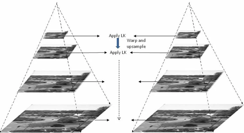
Image pyramid.
Refinement lets us start from an initial estimate. A better initial estimate means a smaller remaining $\Delta d$, less linearization error, and a better final flow estimate.
In an image pyramid, higher levels have lower resolution, so a window of the same size covers a larger area of the real scene. For example, suppose there are three levels: the first has the original resolution, the second is downsampled by 2, and the third by 4. We compute a coarse flow $\Delta d_{l_3}$ at the third level, multiply it by 2, and use it to initialize the second level. Multiply the second-level result by 2 to initialize the first level. The first level produces the final estimate.
Implementation tricks
- Brightness constancy can fail because of illumination changes, camera noise, or viewpoint changes. Histogram equalization is one preprocessing option, though it did not help on my dataset. Tracking consecutive frames also reduces the difference between images. To find flow between the current frame and an older one, we can estimate each consecutive pair and chain the matches: if A = B and B = C, then A = C.
- I did not describe estimation of the affine transformation here, but it may be a better choice. If you implement it, use a larger window because there are more parameters to estimate.
- Surface markings can also fail. One option is to weight window pixels according to image curvature, or discard a window when its intensity is discontinuous.
- Forward-backward tracking can improve precision. After tracking from $I$ to $J$, track the result back from $J$ to $I$. Compare the returned position with the original feature point in $I$; high consistency suggests accurate tracking.
- Classic SLAM systems ORB-SLAM and VINS-Fusion use two different front-end approaches. ORB-SLAM extracts feature descriptors and matches them; VINS-Fusion tracks features with KLT. In a sense, KLT’s descriptor is the raw intensity in the feature’s local window. ORB defines a local-intensity-based descriptor that is more robust to illumination, rotation, translation, and scale. The two approaches have something in common. In my experience, KLT is sufficient in ordinary scenes when camera motion is smooth. Choose according to your own setting.
Experiments
The experimental data came from a video recorded in the lab, with more than a thousand images. I used OpenCV’s built-in function plus forward-backward tracking as ground truth. I also ran ablations on window size, weight $w$, and the image pyramid. The metrics are precision, recall, F1 score, and runtime:
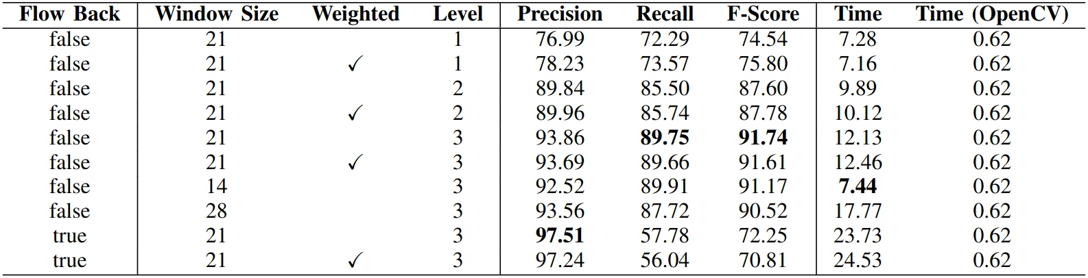
Ablation results.
The image pyramid is the main factor. In fact, pyramids of images or features are a useful tool in computer vision. The weight $w$ seems to help slightly only when the pyramid has few levels. A window size of 21 performs best in this table. I do not know how to determine that value either; OpenCV also defaults to 21, so perhaps it was meant to be.
Forward-backward tracking greatly improves precision and introduces fewer outliers, though recall drops. I would not worry too much as long as there are enough matches; extra matches are not necessarily useful. My implementation is also considerably slower. One reason is that I used bilinear interpolation for both gradients and intensity values to improve accuracy, since the algorithm’s pixel coordinates are floating-point. The other is that I did not use multithreading, so flow is estimated for each feature sequentially.
For practical use, I still recommend OpenCV’s implementation. For coursework, I do not recommend using mine either: the assignment does not require it, and it is not as good as OpenCV’s. As a researcher, though, you can enjoy implementing a classic algorithm. The sea of knowledge is vast, and when the tide goes out, only a few pearls remain. Polishing one yourself from the beginning is a worthwhile experience.
References
- 视觉SLAM十四讲 (Fourteen Lectures on Visual SLAM).
- CMU Tracking KLT.
- Shape and Motion from Image Streams: a Factorization Method.
- An Iterative Image Registration Technique with an Application to Stereo Vision.