Ground-Constrained SLAM for Mobile Robots
Zhijian Qiao
This is an English translation of my Chinese article.
Introduction
Ground contact constrains the motion of a ground robot. This prior can be useful for improving SLAM accuracy. Related approaches include:
- Assuming a flat ground plane and imposing a planar constraint, as in VINS on Wheels.
- Assuming the robot is on a plane but applying stricter checks on the ground constraint: GR-Fusion and Ground-SLAM.
- Treating the ground as a manifold: Pose Estimation for Ground Robots: On Manifold Representation, Integration, Re-Parameterization, and Optimization, B-splines for Purely Vision-based Localization and Mapping on Non-holonomic Ground Vehicles, and Vision-Aided Localization for Ground Robots.
- Incorporating vehicle kinematics: Visual-Inertial Localization for Skid-Steering Robots with Kinematic Constraints.
The ground-plane assumption
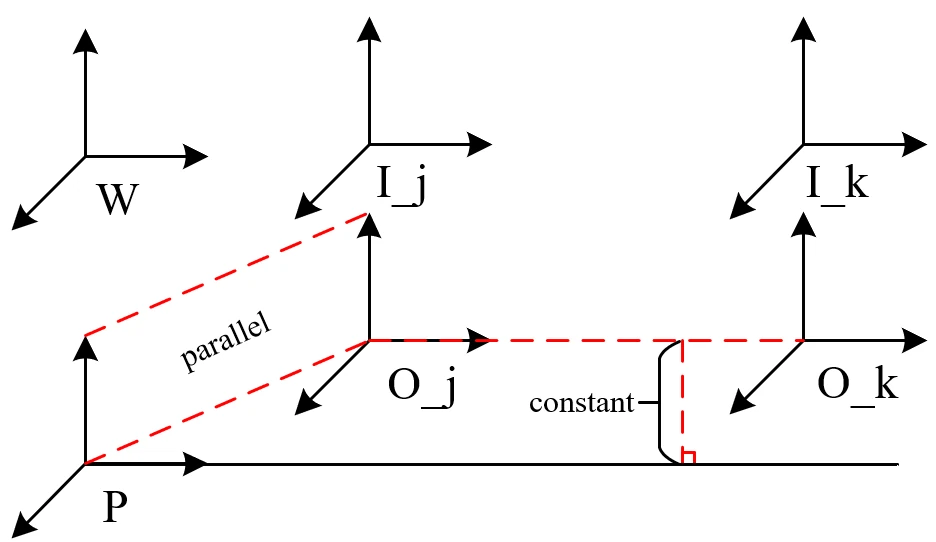
Figure from the Chinese article.
The figure shows six coordinate frames in a typical visual-inertial-wheel (VIW) system: the world frame W, ground-plane frame P, IMU frame $I_j$ and wheel-odometer frame $O_j$ at time j, and IMU frame $I_k$ and odometer frame $O_k$ at time k. We can choose P during initialization; for example, use the initial odometer frame, assuming all four wheels are firmly on the ground. P represents a two-dimensional plane, so its representation differs from those of the other frames. See plane feature parameterization in SLAM for more on plane parameters.
Here we represent P by $R_w^p$ (represented using SO(3), but updated using SO(2)) and $z^p_{O_{init}}$ (a scalar: the initial O-frame z coordinate in P). The ground constraint has two parts: (1) the z axes of P and O remain parallel, and (2) the distance from O to the XY plane of P remains constant.
Following this definition, we can construct the residual:
\[r_{3 \times 1}=\left[\begin{array}{cr} {\left[\begin{array}{ll} \mathbf{e}_{1} & \mathbf{e}_{2} \end{array}\right]^{T} \left(R_{O}^{I}\right)^{T} \left(R_{I_{k}}^{w}\right)^{T} \left(R_{w}^{p}\right)^{T} \mathbf{e}_{3}} \\ \mathbf{e}_{3}^{T} R_{w}^{p}\left(R_{I_{k}}^{w} t_{O}^{I}+t_{I_{k}}^{w}\right)-z_{O_{\text {init }}}^{p} \end{array}\right]=\mathbf{0}\]The state variables to update include the VIW system rotation $R_{I_{k}}^{w}$ and translation $t_{I_{k}}^{w}$, extrinsic rotation $R_{O}^{I}$ and translation $t_{O}^{I}$ between I and O, and P’s rotation $R_{w}^{p}$ and translation $z_{O_{\text {init }}}^{p}$.
Before deriving the Jacobians, let us review some Lie-group identities:
\[[\mathbf{Ra}]_{\times}=\mathbf{R}[\mathbf{a}]_{\times}\mathbf{R}^T\] \[\begin{aligned} \mathbf{J}_{\mathrm{R}}^{\mathrm{R}^{-1}} &=-\mathbf{A} \mathbf{d}_{\mathrm{R}}=-\mathbf{R} \\ \mathbf{J}_{\mathrm{QR}}^{\mathrm{QR}} &=\mathbf{A} \mathbf{d}_{\mathrm{R}}{ }^{-1}=\mathbf{R}^{\top} \\ \mathbf{J}_{\mathrm{R}}^{\mathrm{QR}} &=\mathbf{I} \end{aligned}\] \[\begin{array}{r} \mathbf{J}_{\mathrm{R}}^{\mathrm{R} \cdot \mathbf{v}} \triangleq \lim _{\boldsymbol{\theta} \rightarrow 0} \frac{(\mathbf{R} \oplus \boldsymbol{\theta})_{\mathbf{v}}-\mathbf{R} \mathbf{v}}{\boldsymbol{\theta}}= \\ \lim _{\boldsymbol{\theta} \rightarrow 0} \frac{\mathbf{R} \operatorname{Exp}(\boldsymbol{\theta}) \mathbf{v}-\mathbf{R} \mathbf{v}}{\boldsymbol{\theta}}=\lim _{\boldsymbol{\theta} \rightarrow 0} \frac{\mathbf{R}\left(\mathbf{I}+[\boldsymbol{\theta}]_{\times}\right) \mathbf{v}-\mathbf{R v}}{\boldsymbol{\theta}} \\ =\lim _{\boldsymbol{\theta} \rightarrow 0} \frac{\mathbf{R}[\boldsymbol{\theta}]_{\times} \mathbf{v}}{\boldsymbol{\theta}}=\lim _{\boldsymbol{\theta} \rightarrow 0} \frac{-\mathbf{R}[\mathbf{v}]_{\times} \boldsymbol{\theta}}{\boldsymbol{\theta}}=-\mathbf{R}[\mathbf{v}]_{\times} \end{array}\] \[\mathbf{J}_{\mathbf{v}}^{\mathbf{R} \cdot \mathbf{v}} \triangleq \lim _{\partial \mathbf{v} \rightarrow 0} \frac{\mathbf{R}(\mathbf{v}+\partial \mathbf{v})-\mathbf{R} \mathbf{v}}{\partial \mathbf{v}}=\mathbf{R}\]Here Q and R are rotation matrices, a and v are vectors, Ad denotes the adjoint, and J denotes a Jacobian. See A Micro Lie Theory for State Estimation in Robotics for derivations.
The first two residual components have the following Jacobian with respect to VIW rotation $R_{I_{k}}^{w}$, denoted $\mathbf{J}_{R_{{{I}_{k}}}^{w}}^{{{r}_{2\times 1}}}$:
\[\begin{array}{l} \mathbf{J}_{R_{{{I}_{k}}}^{w}}^{{{r}_{2\times 1}}}=\frac{\partial\left[\begin{array}{ll} \mathbf{e}_{1} & \mathbf{e}_{2} \end{array}\right]^{T}\left(R_{O}^{I}\right)^{T}\left(R_{I_{k}}^{w}\right)^{T}\left(R_{w}^{p}\right)^{T} \mathbf{e}_{3}}{\partial R_{I_{k}}^{w}}\\ =\frac{\partial\left[\begin{array}{ll} \mathbf{e}_{1} & \mathbf{e}_{2} \end{array}\right]^{T}\left(R_{O}^{I}\right)^{T}\left(R_{I_{k}}^{w}\right)^{T}\left(R_{w}^{p}\right)^{T}\mathbf{e}_{3}}{\partial\left(R_{I_{k}}^{w}\right)^{T}\left(R_{w}^{p}\right)^{T} \mathbf{e}_{3}} \times \frac{\partial\left(R_{I_{k}}^{w}\right)^{T}\left(R_{w}^{p}\right)^{T} \mathbf{e}_{3}}{\partial\left(R_{I_{k}}^{w}\right)^{T}\left(R_{w}^{p}\right)^{T}} \times \frac{\partial\left(R_{I_{k}}^{w}\right)^{T}\left(R_{w}^{p}\right)^{T}}{\partial\left(R_{I_{k}}^{w}\right)^{T}} \times \frac{\partial\left(R_{I_{k}}^{w}\right)^{T}}{\partial R_{I_{k}}^{w}}\\ =\left[\begin{array}{ll} \mathbf{e}_{1} & \mathbf{e}_{2} \end{array}\right]^{T}\left(R_{O}^{I}\right)^{T} \times\left(-\left(R_{I_{k}}^{w}\right)^{T}\left(R_{w}^{p}\right)^{T}\left[\mathbf{e}_{3}\right]_{\times}\right) \times R_{w}^{p} \times\left(-R_{I_{k}}^{w}\right)\\ =\left[\begin{array}{ll} \mathbf{e}_{1} & \mathbf{e}_{2} \end{array}\right]^{T}\left(R_{O}^{I}\right)^{T} \times\left(\left(R_{w}^{p} R_{I_{k}}^{w}\right)^{T}\left[\mathbf{e}_{3}\right]_{\times}\left(R_{w}^{p} R_{I_{k}}^{w}\right)\right)\\ =\left[\begin{array}{ll} \mathbf{e}_{1} & \mathbf{e}_{2} \end{array}\right]^{T}\left(R_{O}^{I}\right)^{T}\left[\left(R_{w}^{p} R_{I_{k}}^{w}\right)^{T} \mathbf{e}_{3}\right]_{\times} \end{array}\]Similarly, we obtain $\mathbf{J}_{R_{{w}}^{p}}^{{{r}_{2\times 1}}}$:
\[\begin{array}{l} \mathbf{J}_{R_{w}^{p}}^{r_{2\times1}}=\frac{\partial\left[\begin{array}{ll} \mathbf{e}_{1} & \mathbf{e}_{2} \end{array}\right]^{T}\left(R_{O}^{I}\right)^{T}\left(R_{I_{k}}^{w}\right)^{T}\left(R_{w}^{p}\right)^{T} \mathbf{e}_{3}}{\partial R_{w}^{p}}\\ =\left[\begin{array}{ll} \mathbf{e}_{1} & \mathbf{e}_{2} \end{array}\right]^{T}\left(R_{O}^{I}\right)^{T} \times\left(-\left(R_{I_{k}}^{w}\right)^{T}\left(R_{w}^{p}\right)^{T}\left[\mathbf{e}_{3}\right]_{x}\right) \times \frac{\partial\left(R_{I_{k}}^{w}\right)^{T}\left(R_{w}^{p}\right)^{T}}{\partial\left(R_{w}^{p}\right)^{T}} \times \frac{\partial\left(R_{w}^{p}\right)^{T}}{\partial R_{w}^{p}}\\ =\left[\begin{array}{ll} \mathbf{e}_{1} & \mathbf{e}_{2} \end{array}\right]^{T}\left(R_{O}^{I}\right)^{T} \times\left(-\left(R_{I_{k}}^{w}\right)^{T}\left(R_{w}^{p}\right)^{T}\left[\mathbf{e}_{3}\right]_{\times}\right) \times\left(-R_{w}^{p}\right)\\ =\left[\begin{array}{ll} \mathbf{e}_{1} & \mathbf{e}_{2} \end{array}\right]^{T}\left(R_{O}^{I}\right)^{T} \times\left(R_{I_{k}}^{w}\right)^{T} \times\left(\left(R_{w}^{p}\right)^{T}\left[\mathbf{e}_{3}\right]_{\times}\left(R_{w}^{p}\right)\right)\\ =\left[\begin{array}{ll} \mathbf{e}_{1} & \mathbf{e}_{2} \end{array}\right]^{T}\left(R_{O}^{I}\right)^{T}\left(R_{I_{k}}^{w}\right)^{T}\left[\left(R_{w}^{p}\right)^{T} \mathbf{e}_{3}\right]_{\times} \end{array}\]Although P’s rotation $R_w^p$ has three degrees of freedom, we update only two to avoid overparameterization. For example, set the last column of this 2×3 matrix to zero, and set the corresponding yaw to zero when initializing $R_w^p$.
Similarly, for $\mathbf{J}_{R_{O}^{I}}^{r_{2\times1}}$:
\[\begin{array}{l} \mathbf{J}_{R_{O}^{I}}^{r_{2\times1}}=\frac{\partial\left[\mathbf{e}_{1} \quad \mathbf{e}_{2}\right]^{T}\left(R_{O}^{I}\right)^{T}\left(R_{I_{k}}^{w}\right)^{T}\left(R_{w}^{p}\right)^{T} \mathbf{e}_{3}}{\partial R_{O}^{I}} \\ =\left[\begin{array}{ll} \mathbf{e}_{1} & \mathbf{e}_{2} \end{array}\right]^{T} \times \frac{\partial\left(R_{O}^{I}\right)^{T}\left(R_{I_{k}}^{w}\right)^{T}\left(R_{w}^{p}\right)^{T} \mathbf{e}_{3}}{\partial\left(R_{O}^{I}\right)^{T}} \times \frac{\partial\left(R_{O}^{I}\right)^{T}}{\partial R_{O}^{I}} \\ =\left[\begin{array}{ll} \mathbf{e}_{1} & \mathbf{e}_{2} \end{array}\right]^{T} \times\left(-\left(R_{O}^{I}\right)^{T}\left[\left(R_{I_{k}}^{w}\right)^{T}\left(R_{w}^{p}\right)^{T} \mathbf{e}_{3}\right]_{\times}\right) \times\left(-R_{O}^{I}\right) \\ =\left[\begin{array}{ll} \mathbf{e}_{1} & \mathbf{e}_{2} \end{array}\right]^{T}\left[\left(R_{O}^{I}\right)^{T}\left(R_{I_{k}}^{w}\right)^{T}\left(R_{w}^{p}\right)^{T} \mathbf{e}_{3}\right]_{\times} \end{array}\]Finally, the Jacobians of the last residual component with respect to each optimization variable are:
\[\mathbf{J}_{R_{I_{k}}^{w}}^{r_{1\times1}}=\frac{\partial\left(\mathbf{e}_{3}^{T} R_{w}^{p}\left(R_{I_{k}}^{w} t_{O}^{I}+t_{I_{k}}^{w}\right)-z_{O_{\text{init}}}^{p}\right)}{\partial R_{I_{k}}^{w}}=-\mathbf{e}_{3}^{T} R_{w}^{p} R_{I_{k}}^{w}\left[t_{O}^{I}\right]_{\times}\] \[\mathbf{J}_{t_{t_{k}}^{w}}^{r_{1\times1}}=\frac{\partial\left(\mathbf{e}_{3}^{T} R_{w}^{p}\left(R_{I_{k}}^{w} t_{O}^{I}+t_{I_{k}}^{w}\right)-z_{O_{\text {init}}}^{p}\right)}{\partial t_{I_{k}}^{w}}=\mathbf{e}_{3}^{T} R_{w}^{p}\] \[\mathbf{J}_{t_{O}^{I}}^{r_{1\times1}}=\frac{\partial\left(\mathbf{e}_{3}^{T} R_{w}^{p}\left(R_{I_{k}}^{w} t_{O}^{I}+t_{I_{k}}^{w}\right)-z_{O_{\mathrm{init}}}^{p}\right)}{\partial t_{O}^{I}}=\mathbf{e}_{3}^{T} R_{w}^{p} R_{I_{k}}^{w}\] \[\mathbf{J}_{R_{w}^{p}}^{r_{1\times1}}=\frac{\partial\left(\mathbf{e}_{3}^{T} R_{w}^{p}\left(R_{I_{k}}^{w} t_{O}^{I}+t_{I_{k}}^{w}\right)-z_{O_{\text {init }}}^{p}\right)}{\partial R_{w}^{p}}=-\mathbf{e}_{3}^{T} R_{w}^{p}\left[R_{I_{k}}^{w} t_{O}^{I}+t_{I_{k}}^{w}\right]_{\times}\] \[\mathbf{J}_{z_{O_{\text {init }}}^{p}}^{r_{1\times1}}=\frac{\partial\left(\mathbf{e}_{3}^{T} R_{w}^{p}\left(R_{I_{k}}^{w} t_{O}^{I}+t_{I_{k}}^{w}\right)-z_{O_{\text {init }}}^{p}\right)}{\partial z_{O_{\text {init }}}^{p}}=-1\]